With the rise of big data, new techniques are needed to run statistics and machine learning algorithms efficiently. The goal of a statistics or machine learning algorithm is usually to minimize some objective function by finding the best among a set of possible solutions. For example, running a linear regression requires finding the line that minimizes the distance from the set of points in the dataset to that line. But finding such a solution can be computationally expensive, especially with massive datasets — the runtime for many statistics and machine learning algorithms is a polynomial function of the size of the dataset for some polynomial with degree \(>1\). This fundamental limitation of algorithms on large datasets raises a question: how can we reduce the size of the dataset while approximating the objective function as if it were evaluated on the full data?

Since many algorithms require computing the objective function many times to find the optimal solution, it is often significantly faster to find a coreset and run the algorithm on it than to run the algorithm on the full data.

In the last several decades, coresets have been developed as an answer to this question. A coreset is a weighted subset of a dataset that approximates the full data with respect to a certain objective function or class of objective functions; coresets can be constructed such that the objective function evaluated on the coreset approximates that of the full data. Since many algorithms require computing the objective function many times to find the optimal solution, it is often significantly faster to find a coreset and run the algorithm on it than to run the algorithm on the full data.

Coresets also come with privacy and efficiency benefits for the transfer of data within or between organizations. If an organization needs to share sensitive or proprietary data with a third party, coresets can reduce the total amount of data necessary to transfer and limit the number of individuals affected by a data breach. Especially under data privacy regulations like the EU’s GDPR, where fines are based on the amount of data that was compromised, coresets can reduce the risks of sharing data with third parties. It is also possible to create private coresets, which come with stronger privacy protections.

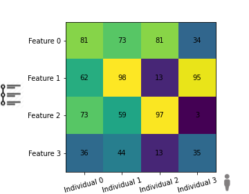
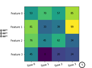
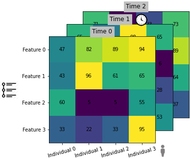
A new paper to be published at NeurIPS 2020 from Lingxiao Huang (a recent postdoc at Yale), K. Sudhir (Yale School of Management) and Nisheeth Vishnoi (Yale Computer Science) shows how to construct coresets for several types of regression objective functions on panel data. Panel data comes from repeated observations of multiple entities (individuals, firms, etc.) over time. We can think of panel data as a combination of two categories of data: cross-sectional data, where a number of entities are measured once, and time-series data, where one entity is measured repeatedly over time. In each of these categories of data, each observation consists of \(d\) features. Coresets for cross-sectional and time-series data have been studied extensively in the literature, but until the new paper, this work had not been extended to the panel data setting. Finding coresets for panel data is challenging because the number of individuals \(N\) and the number of observations per individual \(T\) can be very large, unlike in cross-sectional data, where only \(N\) can be large, or time-series data, where only \(T\) can be large.

Cross-sectional data	Time-series data	Panel data

Cross-sectional data contains features of multiple entities measured once; time-series data contains features of one entity measured over multiple time points; panel data contains features of multiple entities measured over multiple time points.

In the next section, we’ll discuss the utility of coresets for algorithms on big data and intuition for how we might construct them. Then we’ll review the three types of regression objective functions on panel data for which constructing coresets is newly possible: ordinary least squares, generalized least squares, and a clustering extension of generalized least squares. Next, we’ll discuss the main proof techniques behind the new research and, finally, analyze how well the algorithms for finding coresets for regression on panel data perform in practice.

Why are coresets useful, and how do we find them?

There are two primary characteristics of coresets that make them useful.

1. They come with provable guarantees about how well they will approximate the full data. Coresets come with a parameter \(\varepsilon\) which acts as a “knob” controlling how closely the coreset must approximate the full data; the objective function on the coreset will be within a factor of \((1 \pm \varepsilon)\) of the value for the full data. For example, you might choose \(\varepsilon = 0.01\) if you wanted the objective function to be within 1% of the solution on the full data.

2. They are small and fast to compute. The size of a coreset (usually) depends on the desired accuracy \(\varepsilon\) (smaller \(\varepsilon\) requires a larger coreset), but not the size of the data. This means that they can represent very large datasets with only a tiny subset of points. They also generally take linear time in the size of the data to construct; as the number of data points grows, the runtime to find the coreset grows linearly with the size of the input. By contrast, the runtime for many statistics and machine learning problems grows polynomially (for some polynomial with degree \(>1\)) with the size of the data. This means that it is often significantly faster to find the coreset and run the algorithm (perhaps evaluating the objective multiple times) on the coreset than to run the algorithm on the full data.

An important limitation of coresets is that the coreset produced for a particular objective function does not come with any guarantees about other problems. Thus, using a coreset constructed to approximate the full data for a different problem may yield misleading results — coresets are not necessarily good general-purpose summaries of data. Similarly, coresets are not necessarily designed for circumstances when the number of features per observation \(d\) is very large; instead, tools from dimensionality reduction would be more appropriate.

(a) Example data set	(b) Sampling distribution	(c) Coreset

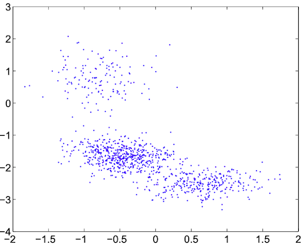
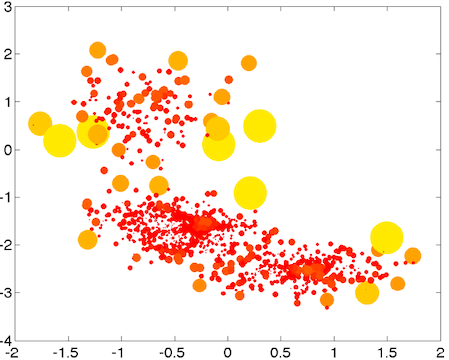
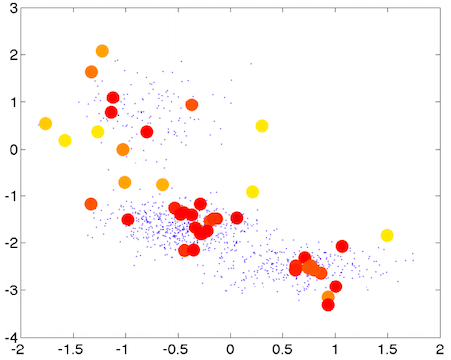
An example process for constructing a coreset.The small blue dots are the original data. For the large yellow/red dots, larger circles indicate “outliers” and color indicates weight (red = high weight). These plots come from Feldman et al, 2011.

Let’s consider how to separate the data in (a) from the figure above into \(k\)-means clusters for \(k=3\). The objective function measures how far each point is away from a cluster center. When there are many points very close to each other, the idea is that we can “summarize” all of those points by including one or a few of them in the coreset. Whereas, when a point is far away from other points (an outlier), we can’t easily summarize it with other points. This means we want to include outliers in the coreset. Then, to capture the original distribution of data, we weight coreset points from dense clusters more heavily than outliers. See (b) from the figure above: larger circles represent “outliers” and red points indicate higher weight. In (c), we can see the points that were selected as part of the coreset and their corresponding weights.

Next, we review the simple case of linear regression for cross-sectional data.

A refresher on regression

Recall simple linear regression on cross-sectional data: For \(N\) individuals and \(d\) features, the data can be modeled as

\[y_i = x_i^\top \beta + \varepsilon_i\]

where \(y_i \in \mathbb{R}\) are the outcomes, \(x_i \in \mathbb{R}^d\) are the predictors, and \(\varepsilon_i \in \mathbb{R}\) are error terms. The vector \(\beta \in \mathbb{R}^d\) consists of the regression coefficients to be estimated.

Under this model, finding the optimal \(\beta\) reduces to minimizing the objective function

\[\psi (\beta) := \sum_{i \in [N]} ( y_{i} - x_{i}^\top \beta )^2.\]

The vector \(\beta\) that minimizes this function is called the ordinary least squares estimator (OLSE).

Why use OLSE? In this post we study \(\ell_2\) regression, the most common and standard type of regression, which uses the \(\ell_2\) norm as a measure of the distance between a point and the regression line, but there are other forms of linear regression based on regularization or other norms. The OLSE turns out to be the best unbiased linear estimator, if we assume the error terms \(\varepsilon_i\) are uncorrelated, have equal variance, and have expected values of zero.

Regression on panel data

To extend OLSE to the panel data setting, we can simply use \(y_{it}\), \(x_{it}\), and \(\varepsilon_{it}\) for individual \(i\) at time \(t\), and model the data as

\[y_{it} = x_{it}^\top \beta + \varepsilon_{it}\]

and use the objective function

\[\psi (\beta) := \sum_{i \in [N]} \sum_{t \in [T]} ( y_{it} - x_{it}^\top \beta )^2\]

As in the cross-sectional data case, the OLSE for panel data is the best unbiased linear estimator, if we assume error terms \(\varepsilon_{it}\) are uncorrelated, have equal variance, and have expected values of zero. But what if we want to account for correlation between time points within individuals?

One of the common ways to model correlation within individuals is called autocorrelation, in which each error term \(e_{it}\) is partially determined by a weighted sum of up to \(q\) preceding error terms \(e_{i(t-q)}, \dots, e_{i(t-1)}\). For autoregression of order \(q\), there is a vector \(\rho \in \mathbb{R}^q\) such that \(\| \rho \|_2 < 1\) (where \(\| \cdot \|_2\) is the \(\ell_2\) norm) and

\[e_{it} = \sum_{j=1}^{\min\{ t-1, t-q \}} \rho_{j} e_{i(t-j)} + N(0, 1)\]

Then the goal is to minimize the objective function

\[\sum_{i=1}^N (1 - \| \rho \|_2^2)(y_{i1} - x_{i1}^\top \beta)^2 + \sum_{t=2}^T \left( (y_{it} - x_{it}^\top \beta) - \sum_{j=1}^{\min\{ t-1, q \}} \rho_{j} (y_{jt} - x_{jt}^\top \beta) \right)^2\]

over the parameters \(\beta, \rho\). The vectors that minimize this object function are called generalized least squares estimators (GLSE).

A clustering extension of GLSE: As an extension of GLSE, one might want to break individuals into clusters and run generalized least squares regression on the clusters. In this case, there are regression coefficient vectors \(\beta^{(1)}, \dots , \beta^{(k)}\) and \(k\) autocorrelation parameter vectors \(\rho^{(1)}, \dots , \rho^{(k)}\). The objective function for a given individual is

\[(1 - \| \rho^{(\ell)} \|_2^2)(y_{i1} - x_{i1}^\top \beta^{(\ell)})^2 + \sum_{t=2}^T \left( (y_{it} - x_{it}^\top \beta^{(\ell)}) - \sum_{j=1}^{\min\{ t-1, q \}} \rho_{j}^{(\ell)} (y_{jt} - x_{jt}^\top \beta^{(\ell)}) \right)^2\]

for whichever \(\ell\) yields the minimum value of the expression. The clustering extension of the generalized least squares estimator is abbreviated GLSE\(_K\).

The new paper allows the construction of coresets for the regression methods described above on panel data.

The technical ideas behind finding a coreset for regression on panel data

Let’s start with a naive idea for constructing coresets for regression on panel data. We can think of panel data as a union of time-series datasets: each time-series dataset could contain all observations for a single entity \(i\). (We could similarly split the panel dataset into \(T\) cross-sectional datasets by fixing \(t\) in each cross-sectional dataset.) To create a coreset, we could find coresets for each time-series dataset and then join all of the coresets together to construct a panel data coreset. However, this would make the size of the coreset depend on the number of entities \(N\). Since \(N\) can be very large, this is undesirable. (Similarly, if we divide the panel dataset into \(T\) cross-sectional datasets, we could find coresets for each of the cross-sectional datasets and join them to find a panel data coreset. However, this would mean the panel data coreset is dependent on \(T\), which is undesirable.) Huang et al find a coreset construction for which the size of the coreset independent of both \(N\) and \(T\).

Huang et al find a coreset construction for which the size of the coreset independent of both \(N\) and \(T\).

To find coresets for regressions on panel data, Huang et al follow a framework from Feldman and Langberg; the Feldman-Langberg framework makes it much simpler to find coresets. The key insight behind the Feldman-Langberg framework is that the objective function is more “sensitive” to certain data points than others, so we should include those high-sensitivity points in the coreset. (In the clustering example above, we called these high-sensitivity points “outliers”.) This intuition can be made quantitative by defining a sensitivity function.

The sensitivity function for individual \(i\) at time \(t\), intuitively, captures how much influence a point has on the total objective function. Recall that \(\psi(\beta, \rho)\) is the objective function, and let \(\psi_{it}(\beta, \rho)\) be the portion of the objective function due to individual \(i\) at time \(t\) (one element of the sum from the objective functions defined above). Formally, the sensitivity function is an upper bound on the supremum of the individual-time objective function as a proportion of the total objective function over all parameters \(\beta, \rho\):

\[s (i,t) \geq \sup_{\beta, \rho} \frac{\psi_{it} (\beta, \rho)}{\psi (\beta, \rho)}\]

Finding an appropriate sensitivity function for GLSE and GLSE\(_K\) on panel data was one of the main technical contributions of the Huang et al paper. (A suitable sensitivity function for OLSE on panel data already existed in the literature.) This was challenging because the objective function for GLSE and GLSE\(_K\) is non-convex. Solving this problem involves developing a relationship between the sensitivities of GLSE and OLSE, and then using the fact that a suitable sensitivity function for OLSE is known to upper bound the sensitivity function for GLSE. Their proof is analogous for GLSE\(_K\), using the relationship to OLSE\(_K\).

Once the sensitivities of each of the points are known, we must choose points to include in the coreset. For this, we can use importance sampling, which has nice probabilistic properties that help prove the guarantees of the coreset. To create the coreset, we can assign probabilities to points proportional to their sensitivities, and then sample from the resulting distribution.

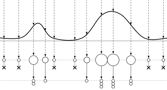
Each point is assigned a probability based on its sensitivity. Points with higher sensitivity are sampled with higher probability. This diagram comes from Happe et al, 2009

Each point is also assigned a weight, which determines how much influence it will have on the algorithm (higher weight = more influence). The weights are generally assigned inversely proportional to sensitivity, such that outliers have the least weight and more representative points have more weight.

It is also important to know how many points to sample from the data. Namely, we need to ensure that the size of the coreset does not depend on \(N\) or \(T\). Huang et al use pseudo-dimension and the total sensitivity (sum of individual sensitivities for each \(i\) and \(t\)) to show that the number of samples needed does not depend on \(N\) or \(T\); together, the pseudo-dimension and total sensitivity upper bound how many points we need to sample, so if the pseudo-dimension does not depend on \(N\) or \(T\), neither does the number of points we need to sample. Pseudo-dimension is a function of the possible inputs, the possible regression parameters and the objective function associated with the analysis.

Next, we discuss how these algorithms perform in practice.

How well does it perform in practice?

Huang et al test their algorithm for constructing coresets on several datasets:

• A synthetic dataset sampled from a multivariate normal distribution.
• A synthetic dataset sampled from a Cauchy distribution, which has heavy tails and undefined expectation and variance. The Cauchy distribution generates “outliers” with greater frequency than the normal distribution - its mean and variance are undefined - and is therefore an interesting test of how the coreset algorithm performs on less well-behaved data.
• A real-world data set of the profits earned from card holders of a credit card company, using individuals’ demographics, past behavior, credit balance and fees paid to predict the profit they might yield.

As a baseline, they compared how the coresets constructed by their algorithm compared to a uniform random sample of the data of the same size as the coreset.

The coreset was able to capture the outliers in the data better than a random sample could.

First, let’s discuss the practical trade-offs between the accuracy parameter \(\varepsilon\) and coreset size. For the synthetic datasets using the normal and Cauchy distributions, the coreset for \(\varepsilon=0.01\) has size less than one half than the full data, while for the \(\varepsilon=0.01\) coreset of the real-world data, the coreset size is about fifth of the size of the original data. The worst-case empirical error for all three tested datasets was always less than the worst-case for uniform random sampling. They also tested \(\varepsilon = 0.2, 0.3, 0.4, 0.5\), which yielded similar patterns. Using \(\varepsilon = 0.5\) yielded a coreset of size less than 1% of the size of the data.

The worst-case error for coresets on the data set generated from the Cauchy distribution were even better than those from the normal distribution, when benchmarked against the uniform random sample: The coreset was able to capture the outliers in the data better than a random sample could.

Next, we can consider how efficient finding and running a regression on the coreset can be compared to running a regression on the full data. On the datasets they tested, finding the coreset and running the regression on it was faster than running the regression on the full data by a factor of 1.2-108x. The computational efficiency of running a regression on the coreset depends on its size, which in turn depends on the accuracy parameter \(\varepsilon\) - so the regression on the coreset is much faster for greater \(\varepsilon\).

You can view their full empirical results in Table 1 of the paper.

Conclusion

Researchers have made rapid progress in expanding the theory of coresets for various statistics and machine learning models. This paper extends the theory of coresets for regression to the panel data setting. The coreset size produced is independent of \(N\) and \(T\) and they show that finding a coreset and running an algorithm on it can be significantly faster than running the algorithm on the full data, in theory and in practice. Panel data is widely used in applications, so this paper presents an exciting contribution to the existing research on the subject. Further, as data regulatory regimes such as the EU’s GDPR and California’s CCPA are developed and implemented, coresets present a convenient way of reducing the risks of data breaches.

Future developments in this area of research may yield new coresets for different problems on panel data relevant in statistics, machine learning, and econometrics.