Over the last decade, increasing attention has been paid to how biased data can impact individuals from marginalized groups. A new paper published last week at the 2020 ICML conference by Elisa Celis, Vijay Keswani (Yale Statistics and Data Science), and Nisheeth Vishnoi (Yale Computer Science) provides a novel pre-processing approach for preventing adverse impacts of biases in data in downstream applications.

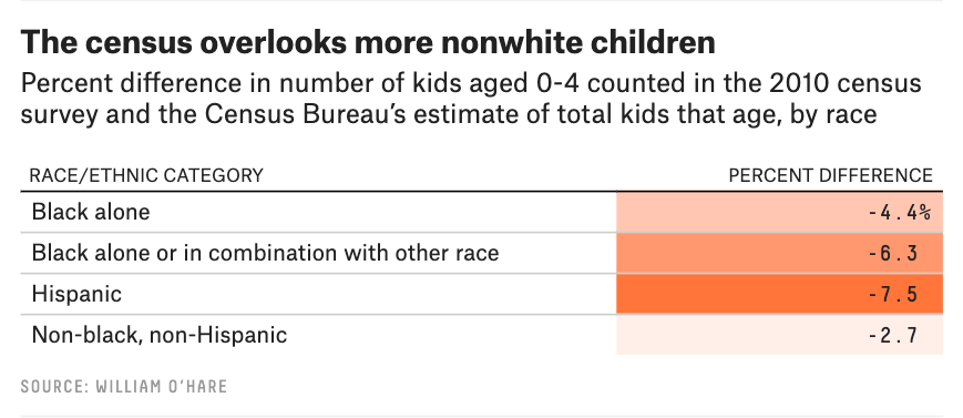
The confluence of two major issues in computation and society motivate this work: the long standing struggle to dismantle discrimination against marginalized groups in society and the rise of data-driven automated decision-making in important social applications. As recently as June, the Supreme Court ruled that the Civil Rights Act of 1964 protects gay, lesbian and transgender employees from discrimination based on sex, extending legal protections related to disparate impact and the 80% rule to the LGBTQ+ community. And yet, major datasets like the U.S. Census can undercount black and Latinx people, leading the government to under-allocate funding for resources needed by those groups (see the infographic from the FiveThirtyEight article below). Additionally, COVID-19 data may be affected by biases; according to FiveThirtyEight, less than half of all data on COVID cases includes race and ethnicity information and news organizations have documented widespread issues with official death counts. Celis et al’s paper provides a new framework for debiasing data and mitigating disparate impact.

According to an analysis by FiveThirtyEight, the Census undercounts black and Latinx children at greater rates than white children.

The main contribution of the paper is a framework for finding a “maximally noncommittal” distribution which closely resembles the distribution induced by the data while ensuring proportionate representation and/or other notions of fairness. And whereas previous similar methods for debiasing data have been prohibitively slow for datasets with large domains, learning the distribution for the new framework can be done efficiently; it takes time polynomial in the dimension of the data.

The methods described in this blog post are preprocessing methods which remove bias from data before machine learning algorithms are trained. However, it should be noted that even if the data is unbiased, there is no guarantee that the algorithm or downstream application will be fair. See this post in Suresh Venkatasubramanian’s Algorithmic Fairness blog for a helpful discussion of this topic. Hence, this is an important step that can be used in conjunction with other tools when designing a just system.

Approaches for debiasing data

In the fairness literature, there are two established approaches for debiasing data: modifying the dataset or learning a fair distribution. Fair data is ensured using fairness constraints, or mathematical statements encoding some formal definition of fairness. See this post for context on many types of fairness constraints.

Following the principle of maximum entropy, the framework produces a max-entropy distribution with a prior distribution determined by reweighting the data points and a carefully chosen marginal to satisfy fairness constraints.

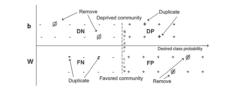
To modify a dataset to satisfy fairness constraints, one can either reassign the protected attributes of some data points or reweight the frequency of data points to satisfy fairness constraints. (See this post for a walkthrough of how this might work in practice.) These approaches are often computationally efficient, but there is no way to generate new data points. As a result, machine learning models trained on the data can fail to generalize. (See Chawla’s “Data mining for imbalanced datasets: An overview” in Data Mining and Knowledge Discovery Handbook for an overview.)

A simple reweighting scheme from (Kamiran and Calders 2012). Some data points are deleted and some data points are duplicated to ensure fairness.

Alternatively, one can learn a distribution which is close to that induced by the data points while satisfying fairness constraints. (See this 2017 paper by Calmon et al for an example of this approach.) This approach allows machine learning models to sample from the learned distribution, with the potential to learn greater generalization from the data. However, past research on fair distributions has produced algorithms which run in time exponential in the dimension of the data; thus, they can be infeasible for large datasets.

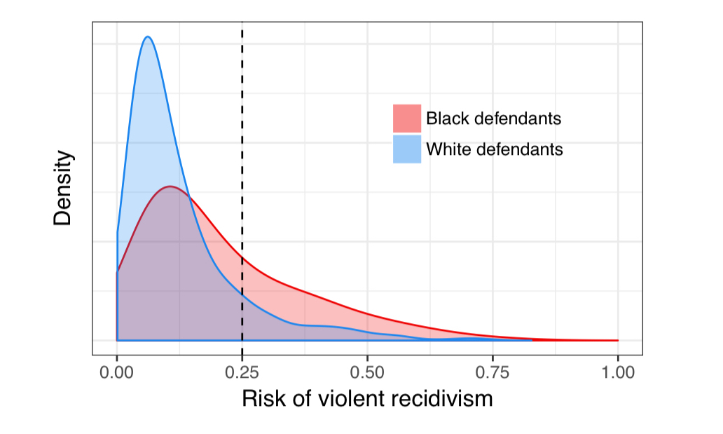
An empirical distribution of violence recidivism by race demonstrating how disparate impacts in algorithmic sentencing decisions might occur. See this excellent blog post for a longer discussion of the need for computing fair distributions.

The algorithm from Celis et al’s paper combines the two approaches above. Following the principle of maximum entropy, the framework produces a max-entropy distribution with a prior distribution determined by reweighting the data points and a carefully chosen marginal to satisfy fairness constraints. It overcomes the infeasibility issues of learned distribution approaches for large datasets by providing an algorithm which runs in time polynomial in the dimension of the dataset.

Next, we discuss the maximum entropy framework, why it is an appealing tool for debiasing data, and how it can be efficiently computed.

Maximum entropy distributions make the fewest assumptions about the data

For a given set of data, there may be many distributions which can encode the data. The principle of maximum entropy says that the distribution with the maximum entropy relative to other possible distributions is the one that best represents the current state of knowledge: it is “maximally noncommittal” in the sense that it makes the fewest assumptions about the true distribution of the data. This principle has its roots in the works of Boltzmann and Gibbs, and E.T. Jaynes, when he was working on questions in statistical physics, first advocated for the approach.

Max-entropy distributions have been studied across many applications as a density estimation method. They also have other desirable properties:

• The number of parameters in a max-entropy distribution is equal to the dimension of the data.
• Maximum entropy distributions are specified by a prior distribution and marginal vector, described in more detail later. The prior and marginal can be viewed as simple, interpretable ways to specify fairness constraints while finding a maximum entropy distribution which is close to the sample data.

Now that we understand some of the desirable properties of the maximum entropy framework, let us go into some of the mathematical specifics of maximum entropy distributions, starting with a definition. For simplicity, we will just discuss the case when the domain \(\Omega\) is \(\{0,1\}^d\).

Finding a maximum entropy distribution

Given prior distribution \(q : \Omega \rightarrow [0, 1]\) and marginal vector \(\theta \in [0,1]^d\), the maximum entropy distribution is the probability distribution which maximizes

$$ \sum_{\alpha \in \Omega} p(\alpha) \log \frac{q(\alpha)}{p(\alpha)}$$

such that \(\sum_{\alpha \in \Omega} \alpha p(\alpha) = \theta\).

The problem stated above is convex, so it can be solved efficiently in the number of parameters. But as the problem is currently stated, there are \(2^d\) parameters. Thus, it could take exponential time in the dimension of the data to solve. To reduce the optimization problem down to polynomial time in the dimension of the data, the problem can be restated as a minimization problem (its dual) with only \(d\) variables:

Dual for finding a maximum entropy distribution

The maximum entropy distribution can be specified by \(d\) parameters \(\lambda \in \mathbb{R}^d\) by finding the minimum of the function

$$ h_{\theta,q} (\lambda) = \log \left( \sum_{\alpha \in \Omega} q(\alpha) e^{\langle \alpha - \theta, \lambda \rangle}\right) $$

Solving this dual optimization problem in polynomial time is non-trivial, but it has been done in recent work. For the sake of brevity, we won’t state the dual or discuss specifics of this problem in this post.

Before we discuss the specifics of the maximum entropy framework can help debias data, we need to review two common fairness metrics.

Fairness metrics: representation and statistical rates

Researchers usually include fairness metrics in debiasing algorithms by considering either outcome independent or dependent constraints. Outcome independent constraints depend only on the protected attributes of the data, while outcome dependent constraints depend on the protected attributes and outcome variables of the data. In the paper, Celis et al consider two well-studied fairness metrics: representation rate, an outcome independent constraint, and statistical rate, an outcome dependent constraint. (Most papers consider just one or the other of these metrics.)

Representation rate

Consider the feature domain \(\Omega = \Omega_1 \times \dots \times \Omega_d = \{0, 1\}^d\). (For simplicity, each attribute \(\Omega_i\) is binary, but these definitions can be adapted to multi-valued discrete attributes.) Partition the attributes into three classes where

• \(I_x\) is the set of protected attributes,

• \(I_y\) is the set of outcome variables,

• and \(I_z\) is the set of other remaining attributes.

For \(\tau \in (0,1]\), a distribution \(p: \Omega \rightarrow [0, 1]\) is said to have representation rate \(\tau\) with respect to a protected attribution \(l \in I_z\) if for all \(z_i, z_j \in \Omega_l\), we have

$$\frac{p[Z=z_i]}{p[Z=z_j]} \geq \tau$$

where \(Z\) is distributed according to the marginal of \(p\) restricted to \(\Omega_l\).

In other words, the representation rate is the outcome-independent ratio of the probability assigned to the under-represented group and the probability assigned to the over-represented group.

Note that all attributes are split into binary categories. One can extend the results to the setting where there are more than two categorical labels by using one-hot encodings. Further, to extend the results to settings with continuous-valued attributes, one could split the range of the continuous attribute into discretized bins with one-hot encodings.

Statistical rate

Define the set of class labels to be \(\mathcal{Y} = \times_{i \in I_y} \Omega_i\). For \(\tau \in (0, 1]\), a distribution \(p : \Omega \rightarrow [0, 1]\) is said to have statistical rate \(\tau\) with respect to a protected attribute \(l \in I_z\) and a class label \(y \in \mathcal{Y}\) if for all \(z_i, z_j \in \Omega_l\), we have

$$ \frac{p\left[Y=y \;\middle|\; Z=z_i \right]}{p\left[Y=y \;\middle|\; Z=z_j \right]} \geq \tau $$

where \(Y\) is the random variable when \(p\) is restricted to \(\mathcal{Y}\) and \(Z\) when \(p\) is restricted to \(\Omega_l\).

Then the statistical rate is the ratio of the probability of belonging to a particular class given the individual is in the under-represented group and the probability of belonging to the same class given the individual is in the over-represented group.

Now, equipped with an understanding of max-entropy distributions and fairness metrics, we can discuss how to satisfy representation and statistical fairness constraints with a carefully chosen prior distribution and marginal vector.

A novel maximum entropy framework for debiasing data

In order to use the maximum entropy framework to debias data, we need a way to encode common fairness constraints like those we defined above. This is the key insight of the maximum entropy design of the debiasing algorithm.

Fairness constraints are specified through the prior distribution and the marginal vector. The prior distribution allows the distribution to satisfy statistical rate constraints, while the marginal vector allows the distribution to satisfy representation rate constraints.

Once we have a prior and marginal vector, it can be shown that the max-entropy distribution resulting from the convex optimization problem above comes with fairness guarantees which are close to those specified by the prior and marginal vector (Theorem 4.5 from the paper). We won’t discuss the bounds or proof in this post.

Choosing a prior distribution

To determine how the prior distribution can satisfy statistical rate constraints, we can first think about the uniform distribution \(u\). Since

$$ u(\alpha) = \frac{1}{|\Omega|} $$

for any \(\alpha\), the statistical rate is

$$ \frac{p\left[Y = y\;\middle|\; Z = z_i\right]}{p\left[Y = y \;\middle|\; Z = z_j\right]} = 1$$

for any class label \(y \in \mathcal{Y}\) and protected attributes \(z_i, z_j \in \Omega_l\) for \(l \in I_z\). Thus, the uniform distribution satisfies \(\tau = 1\) statistical fairness.

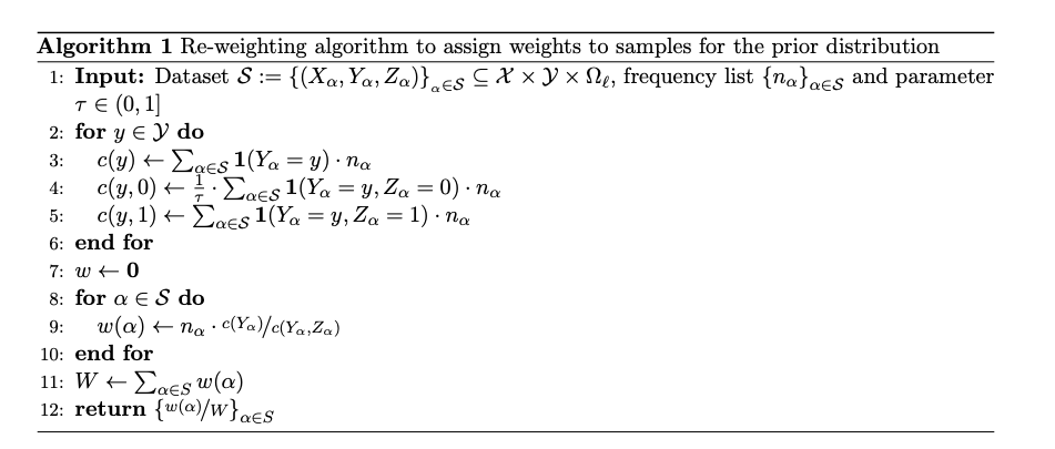
However, the uniform distribution does not encode any information from the sample data. To encode information from the empirical data while preserving \(\tau\)-statistical fairness, Celis et al use a reweighting algorithm. See the figure below from the paper.

Let’s walk through an example to see how it works, using \(\tau = 1\). Consider the figure below.

On the left, the green icons are positive class labels (\(Y=1\)) and the pink icons are negative class labels (\(Y=0\)), while the circled icons are samples from the population. As in the algorithm, denote \(Z=0\) to be the underrepresented group with the female icons and \(Z=1\) to be the overrepresented group with the male icons. We can construct the following table for values of \(c(\cdot)\) and \(c(\cdot, \cdot)\).

Expression	Value	Explanation
\(c(1)\)	3	Count positive class labels from the sampled data
\(c(0)\)	4	Count negative class labels from the sampled data
\(c(1, 1)\)	2	Count male positive class labels from the sampled data
\(c(1, 0)\)	1	Count female positive class labels from the sampled data
\(c(0, 1)\)	2	Count male negative class labels from the sampled data
\(c(0, 0)\)	2	Count female negative class labels from the sampled data

Calculating the value of \(w\) for the female positive class label, we have \(c(1)/c(1,0) = 3\). We can do this for each \(\alpha\) to find the weights shown below.

Notice that the sum of the weights assigned to male and female positive class labels respectively are equal to each other (3 = 1.5 + 1.5). Similarly, the total weight assigned to male and female negative class labels respectively are equal to each other (2 + 2 = 2+ 2). Thus, the ratio of the conditional probabilities is equal to 1:

$$ \frac{p \left[ Y=1 \;\middle|\; Z=0 \right]} {p \left[ Y=1 \;\middle|\; Z=1 \right]} = 1$$

and

$$ \frac{p \left[ Y=0 \;\middle|\; Z=0 \right]} {p \left[ Y=0 \;\middle|\; Z=1 \right]} = 1$$

so the prior distribution has a \(\tau=1\) statistical rate.

One might think that since it satisfies \(\tau\)-statistical fairness and resembles a reweighted version of the sample data, this construction of the prior distribution is itself a sufficient debiasing mechanism. However, finding the max-entropy distribution pushes the distribution towards the empirical distribution of the data while still satisfying fairness constraints.

Choosing the marginal vector

A simple choice for the marginal vector would be the expectation vector \(\theta = \frac{1}{N} \sum_{\alpha \in \mathcal{S}} \alpha n_\alpha\) This would yield a representation rate equivalent to the representation rate of the sample data, since \(\frac{p\left[ Z = z_i \right]}{p[Z = z_j ]}\) for \(i,j \in \Omega_l\) where \(l \in I_z\) would be equivalent to the ratio of that attribute in the sample data.

Celis et al found that the novel max-entropy framework performs as well as or better than existing debiasing methods in finding a distribution close to the data — while attaining good representation and statistical rates simultaneously.

By contrast, setting every entry of the marginal vector to 0.5 would yield a representation rate of 1, since the ratio of marginal probabilities of attributes from one class would be equal to that from the other: the probability of \(Z = 1\) would be 0.5 and the probability of \(Z=0\) would be 0.5. Thus, it is always possible to choose the marginal vector such as to satisfy a \(\tau\)- representation rate for any \(\tau\).

Using the prior distribution and marginal vector, the max-entropy framework is able to satisfy both representation rate and statistical rate fairness constraints.

How well does it do in practice?

The max-entropy framework was evaluated empirically on two benchmark fairness datasets:

• the COMPAS criminal defense dataset, which includes criminal histories jail and prison time, demographics and risk scores according to a commercial risk assessment algorithm for a group of defendants.
• the Adult financial dataset, which includes the demographics of a group of individuals as well as a binary label of whether their income is greater than $50k. They also trained a classifier on the debiased data to report the statistical rates of the classifier.

Celis et al found that the novel max-entropy framework performs as well as or better than existing debiasing methods in finding a distribution close to the data — while attaining good representation and statistical rates simultaneously. Across both of the datasets tested, the statistical rate and representation rate of the computed max-entropy distribution was at least 0.97, very close to the maximum of 1 and higher than the raw data. The classifier trained on the COMPAS dataset lost accuracy by 0.03 compared to the raw data, while the classifier trained on the Adult dataset achieved the same accuracy as the classifier trained on the raw data; these accuracies are the same or better than existing debiasing methods using the same benchmark datasets. See the complete results in the paper for representation rates, data statistical rates, classifier statistical rates, classifier accuracy, and run-times for both datasets.

The code for the algorithm is available on GitHub.

To conclude

Data preprocessing to mitigate bias remains an important task across a range of applications. Celis et al’s paper leverages the maximum entropy framework, using a carefully chosen prior distribution and marginal vector to satisfy fairness constraints and remains close to the empirical distribution induced by the data. Further, their algorithm runs in polynomial time in the dimension of the data, rather than the size of the domain, unlike prior results. A key limitation of the paper, however, is that the framework applies only in discrete domains. Future work might include extending the framework to continuous domains or to include fairness across “intersectional types” so that the data is unbiased for multiple independent protected attributes.

The ICML version of the paper is here and the full version is available on arXiv.